Code
import matplotlib.pyplot as plt
import metropolis_mc
fig, ax = plt.subplots(figsize=(8, 4.2))
metropolis_mc.plot_entropy_vs_energy(ax)
plt.show()Introducing and solving the 2-D Ising Model using a Metropolis Monte Carlo simulation.
Kyle Arean-Raines
September 18, 2026
The Ising Model (Ising 1925) is a model in statistical mechanics that involves - as before - magnetic spins in a lattice. It can describe spontaneous magnetization and phase transitions in magnetic lattices. The one-dimensional lattice with nearest-neighbor interactions is solvable at the graduate level. Many classes on statistical mechanics will go through this. The situation gets vastly more complex when you increase the number of dimensions to two. In fact, it took years before Onsager solved the 2-D model analytically (Onsager 1944).
We’ll use a numerical approach to solving the 2-D Ising model in the absence of an external field. Here, neighboring sites influence each other through an interaction term. The energy of the lattice is a sum over interacting pairs of sites, given by
\[ E_{\text{total}} = -J \sum_{\langle i j \rangle} s_i s_j \]
where \(J\) is a proportionality constant describing the strength of interactions, \(\langle i j \rangle\) means the sum runs over each pair of nearest-neighbor sites exactly once, and \(s_i\) and \(s_j\) take on the values \(\pm 1\) based on whether the spins are aligned or anti-aligned. Counting each pair once is the part worth being careful about: every bond joins two sites, so adding up a per-site energy across the whole lattice would count all of them twice. Note here the absence of an external magnetic field. Contrast that with the previous case of non-interacting spins in a lattice with a field applied.
The approach we’ll take to tackle this problem is called the Metropolis Monte Carlo method (Metropolis et al. 1953), and it allows us to simplify the calculations and numerically solve without doing in-depth calculations (e.g. solving for the partition function). It is probabilistic, in that each step or perturbation in the simulation has some probability of carrying over to the next step based on the energetic “favorability.” That is, for a single spin flip, if it lowers the total energy of the system it is automatically accepted. Whereas if the total energy increases, there is a finite less-than-one probability that we’ll accept the move. As the simulation carries on we get closer to an equilibrium state.
This allows us to calculate macroscopic thermodynamic quantities, such as total energy and magnetization.
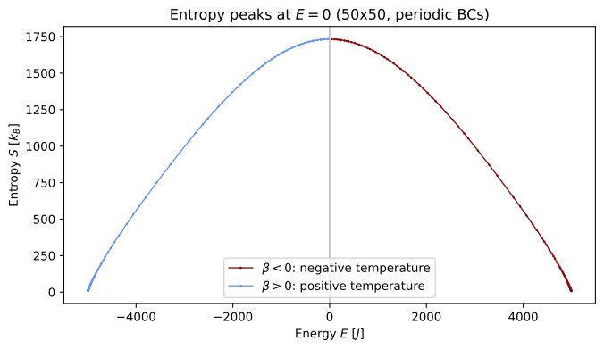
As I’ve shown below by plotting the results of the simulation, we see a similar curve where temperature goes negative as we add more and more energy to the system and as the entropy goes down. The blue branch is the ordinary positive-temperature half of the sweep (\(\beta > 0\)), where entropy climbs as energy is added. The dark red branch is the negative-temperature half (\(\beta < 0\)), past the entropy peak at \(E = 0\), where adding energy leaves the lattice with fewer and fewer states to occupy.
The full source for this series is on GitHub. The derivations, code, and prose are all mine. However, I did consult Claude to proofread and for help setting up the project and rendering equations.
A weekly email if there's something new.
---
title: "Negative temperature part 3: the Ising Model"
description: >
Introducing and solving the 2-D Ising Model using a Metropolis Monte Carlo simulation.
date: 2026-09-18
author: "Kyle Arean-Raines"
categories: [Intermediate, statistical mechanics, Monte Carlo, simulation]
toc: true
bibliography: ../../references.bib
---
# The Ising Model
## Intro
The [Ising Model](https://en.wikipedia.org/wiki/Ising_model) [@ising1925] is a model in statistical mechanics that involves -
as before - magnetic spins in a lattice. It can describe spontaneous magnetization and phase transitions in
magnetic lattices.
The one-dimensional lattice with nearest-neighbor interactions is solvable at the graduate level. Many classes on
statistical mechanics will go through this. The situation gets vastly more complex when you increase the number
of dimensions to two. In fact, it took years before Onsager solved the 2-D model analytically [@onsager1944].
## Numerical methods
We'll use a numerical approach to solving the 2-D Ising model in the absence of an external field. Here, neighboring
sites influence each other through an interaction term. The energy of the lattice is a sum over interacting pairs
of sites, given by
$$
E_{\text{total}} = -J \sum_{\langle i j \rangle} s_i s_j
$$
where $J$ is a proportionality constant describing the strength of interactions, $\langle i j \rangle$ means the sum
runs over each pair of nearest-neighbor sites exactly once, and $s_i$ and $s_j$ take on the values $\pm 1$ based on
whether the spins are aligned or anti-aligned. Counting each pair once is the part worth being careful about: every
bond joins two sites, so adding up a per-site energy across the whole lattice would count all of them twice. Note
here the absence of an external magnetic field. Contrast that with the previous case of non-interacting spins in a
lattice with a field applied.
The approach we'll take to tackle this problem is called the Metropolis Monte Carlo
method [@metropolis1953], and it allows us to simplify the calculations and numerically solve without doing in-depth calculations
(e.g. solving for the partition function). It is probabilistic, in that each step or perturbation in the simulation
has some probability of carrying over to the next step based on the energetic "favorability." That is, for a
single spin flip, if it lowers the total energy of the system it is automatically accepted. Whereas if the total
energy increases, there is a finite less-than-one probability that we'll accept the move. As the simulation carries
on we get closer to an equilibrium state.
This allows us to calculate macroscopic thermodynamic quantities, such as total energy and magnetization.
## Results
As I've shown below by plotting the results of the simulation, we see a similar curve where temperature goes negative
as we add more and more energy to the system and as the entropy goes down. The blue branch is the ordinary
positive-temperature half of the sweep ($\beta > 0$), where entropy climbs as energy is added. The dark red branch
is the negative-temperature half ($\beta < 0$), past the entropy peak at $E = 0$, where adding energy leaves the
lattice with fewer and fewer states to occupy.
```{python}
#| label: fig-interacting-lattice
#| fig-cap: "Entropy vs. energy for the 2-D Ising Model."
#| code-fold: true
import matplotlib.pyplot as plt
import metropolis_mc
fig, ax = plt.subplots(figsize=(8, 4.2))
metropolis_mc.plot_entropy_vs_energy(ax)
plt.show()
```
## References
::: {#refs}
:::
The full source for this series is on
[GitHub](https://github.com/kareanra/physics-blog).
The derivations, code, and prose are all mine. However, I did consult Claude to proofread and for help
setting up the project and rendering equations.