Negative temperature part 2: an exact solution to the spin lattice

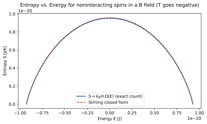
Extending the discussion from part 1 and coming up with an analytical solution for entropy as a function of energy. This demonstrates temperature going negative quantitatively.

Revisiting the spin lattice

Intro

Last post we talked about the lattice or “grid” of magnets (spins) in an externally-applied field. We saw that for the case of our system, there’s a point above which further increasing the energy of the system forces it into lower-entropy states. Hence, the sign of temperature goes negative. We’ll show that quantitatively in this post, deriving the entropy as a function of energy, and plotting our result to see that the slope goes negative. To follow these calculations, it helps to have some knowledge of statistical mechanics, though a solid math background would probably suffice.

Calculating the energy

In the last post we calculated the energy of a noninteracting system of spins in a B field. It’s just

\[ E = - \sum_{i = 1}^{N} \mu s_i B = -\mu B (N_\uparrow - N_\downarrow) \]

where the sum runs over all spins in the lattice, and in the rightmost expression the \(N\)s describe the number of spins in that orientation. The fully-aligned state has the lowest energy

\[ E = -N \mu B \]

and has an entropy of exactly 0 since there is only one way to orient all the spins along B.

The maximum energy is \(E = N \mu B\) with all spins anti-aligned and entropy 0. The energy calculation is therefore very straightforward.

Calculating the entropy

We alluded to the entropy being related to or proportional to the number of ways to achieve a state by rearranging and flipping spins in the lattice. The exact definition we’ll use is

\[ S = k_B \ln \Omega(E) \]

where \(k_B\) is Boltzmann’s constant (just a number), \(\ln\) is the natural logarithm, and \(\Omega\) is the number of states corresponding to a particular energy. For our spin system

\[ \Omega = C(N, N_\uparrow) = {N \choose N_\uparrow} = \frac{N!}{N_\uparrow! N_\downarrow!} \]

The \(N\)s in the binomial coefficient above correspond to the number of spins in the up or down state. The total expression reflects the fact that we have a two-level system: it’s the same as if you were to pick balls randomly from a bucket of red and blue balls.

Okay now back to entropy. The entropy of our system is

\[ S = k_B \ln \frac{N!}{N_\uparrow! (N - N_\uparrow)!} = k_B \ln(N!) - k_B \ln (N_\uparrow!) - k_B \ln \big((N - N_\uparrow)!\big) \]

To slightly simplify our calculations we’ll now apply Stirling’s approximation for factorials:

\[ \ln (N!) \approx N \ln N - N \]

\[ S = N k_B \ln N - N_\uparrow k_B \ln N_\uparrow - N_\downarrow k_B \ln N_\downarrow - k_B(N - N_\uparrow - N_\downarrow) \]

The last term is clearly zero, which leaves

\[ S = N k_B \ln N - N_\uparrow k_B \ln N_\uparrow - N_\downarrow k_B \ln N_\downarrow \] \[ = k_B \left[N \ln N - N_\uparrow \ln N_\uparrow - (N - N_\uparrow) \ln (N - N_\uparrow) \right] \]

Then invert the energy expression above, \(E = -\mu B (N_\uparrow - N_\downarrow)\) to get \(N_\uparrow(E)\):

\[ N_\uparrow = \frac{N}{2} \left( 1 - \frac{E}{N \mu B} \right) \]

And finally substituting into the entropy equation we get

\[ S(E) = -N k_B \left[ \frac{N\mu B - E}{2N\mu B} \ln\!\left(\frac{N\mu B - E}{2N\mu B}\right) + \frac{N\mu B + E}{2N\mu B} \ln\!\left(\frac{N\mu B + E}{2N\mu B}\right) \right] \]

That’s a lot of terms, but it’s a closed form solution to the problem, which is exceedingly rare and breaks down for the vast majority of interacting systems. Now let’s plot this to show that inverted-dome shape relationship where T goes negative.

import matplotlib.pyplot as plt
import noninteracting_lattice

fig, ax = plt.subplots(figsize=(8, 4.2))
noninteracting_lattice.plot_entropy_vs_energy(ax)
plt.show()

Figure 1: Entropy vs. energy for a noninteracting spin lattice in a B field. The solid curve counts the microstates exactly, \(S = k_B \ln \Omega\); the dashed curve is the closed form we just derived. They are indistinguishable except within a few spin flips of either end, where Stirling’s approximation is being applied to \(\ln(1!)\).

fig, ax = plt.subplots(figsize=(8, 4.2))
noninteracting_lattice.plot_inverse_temperature_vs_energy(ax)
plt.show()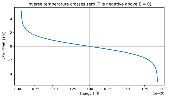

Figure 2: Inverse temperature \(1/T = dS/dE\) across the same energy range. It crosses zero at \(E = 0\) and is negative for every energy above it.

In part 3 we’ll deal with interacting spins with no external field applied. Stay tuned!

The full source for this series is on GitHub. The derivations, code, and prose are all mine. However, I did consult Claude to proofread and for help setting up the project and rendering equations.