Code
import matplotlib.pyplot as plt
import dslit

fig, ax = plt.subplots(figsize=(8, 4.2))
dslit.draw_schematic(ax)
plt.show()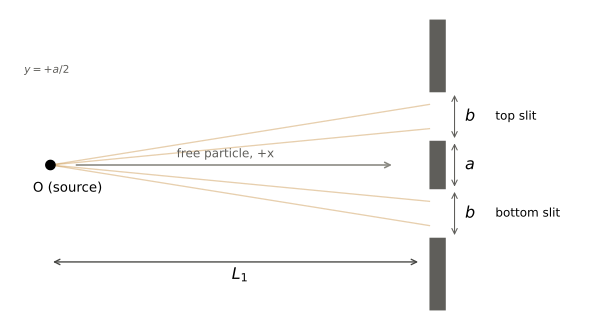
Solving the Schrödinger equation for a Gaussian wave packet incident on two Gaussian-aperture slits, deriving a closed-form interference pattern via complex Gaussian integrals, and checking the predicted fringe spacing numerically.
Now let’s get our hands dirty with some math and code. Again, this is pretty advanced stuff, so feel free to skip to the diagrams showing the interference results.
Prerequisites: differential equations, Fourier transforms, Gaussian integrals, vector calculus, and perhaps some basic physics.
Though two of three grad courses I took on quantum mechanics referenced this experiment, the treatment was mostly qualitative, even though rigorous mathematical machinery was subsequently developed throughout the course. Further, we didn’t do much until Quantum II involving path integrals, which is an alternative way of formulating quantum that typically isn’t taught in introductory classes on the subject. But this double-slit problem is actually relatively tractable using this alternative framework. We’ll get to that after walking through some derivations using the Schrödinger approach.
The Schrödinger equation is a second-order partial differential equation that describes the time evolution of a quantum system. In classical mechanics, using the Euler-Lagrange equations gives you a deterministic trajectory of a particle or system through space and time. If you know the initial state of the system at a given time, you can calculate the system state at any subsequent time, provided you know the form of the Lagrangian (energy “function” for the environment the system is in).
In quantum mechanics, there is no such determinism. It is the probabilities of the state being in a state at a given time that evolve according to the equations of “motion.” So here’s the famous Schrödinger equation, (technically speaking, the position- or space-representation of the general equation):
\[ i \hbar {\frac {\partial^2 \Psi(\mathbf{r}, t)}{\partial t^2}} = \frac{-\hbar^2}{2m} \nabla^2 \Psi(\mathbf{r}, t) + V (\mathbf{r}, t) \Psi(\mathbf{r}, t) \]
where \(\Psi\) is the wavefunction, which varies in space and time and \(V(\mathbf{r}, t)\) is the potential energy. The wavefunction describes the probability of finding a particle at a given point in space at a given time.
In any graduate textbook on quantum theory, you’ll find a solution to the Schrödinger equation that is a wave “packet.” This is a wavefunction \(\Psi(x, t)\) that has the form of a Gaussian (\(\propto e^{\alpha x^2}\)). In other words, the wavefunction is slightly spread out over space rather than all the probability being concentrated at a point. You can get some cool intuition and solve more problems with this type of wavefunction. Aside: it’s also easy to demonstrate the relationship between position uncertainty and momentum uncertainty with such a wave packet.
Question for the reader: How would you show that relationship using a wave packet? (Hint: the momentum space wavefunction is essentially obtained through a Fourier transform of the [Gaussian] position wavefunction, and describes how spread out the momentum is - with more spread out being higher uncertainty).
That this solves the Schrödinger equation can be easily shown. You can find the derivation in most graduate texts, including Cohen-Tannoudji et al. (1977).
I recently dusted off Feynman and Hibbs’ Quantum Mechanics and Path Integrals (Feynman and Hibbs 1965), a fascinating treatment of quantum mechanics that doesn’t use much of the linear algebra and operator-based formulation. The core idea here (without regurgitating everything) is that there is a cool, different way of calculating the probability amplitude of a particle that starts at \((x_0, t_0)\) in spacetime arriving at \((x_1, t_1)\).
The propagator for a free particle (that which is traveling through space with no potential anywhere) is defined as follows (presented without justification; see Feynman and Hibbs):
\[ K(x_b, t_b; x_a, t_a) = \sqrt{\frac{m}{2\pi i \hbar (t_b - t_a)}}\; \exp\!\left[\frac{i m (x_b - x_a)^2}{2\hbar (t_b - t_a)}\right] \]
This happens to be exactly what we’re looking for - the propagator tells us the probability of arriving at the top or bottom slit at a given time, and then due to its linearity can be multiplied and integrated with the propagator for the particle starting at either slit and arriving at some point on the detector screen.
So without further ado, let’s jump into the math.
Now we have a solution that models a particle in real space, slightly spread out, and which solves the Schrödinger equation. Let’s make all this concrete with our experiment. A free electron leaves the origin traveling in \(+x\) toward a screen a distance \(L_1\) away. The screen has two slits: the top slit spans \(y \in [+a/2,\, +a/2+b]\) and the bottom slit \(y \in [-a/2-b,\, -a/2]\), so the central barrier between them has height \(a\) and each opening has height \(b\).
import matplotlib.pyplot as plt
import dslit
fig, ax = plt.subplots(figsize=(8, 4.2))
dslit.draw_schematic(ax)
plt.show()Here we let the transmitted wave keep going to a detection screen a distance \(L_2\) beyond the slits and derive the interference pattern in closed form. The trick is to model each slit as a Gaussian aperture. A Gaussian packet times a Gaussian slit is still Gaussian, and free evolution using the propagator maps Gaussians to Gaussians, so every step stays analytic and no grid is needed.
Throughout, \(y\) is the transverse coordinate and the along-axis drift is just the time axis. The packet reaches the slits at \(t_1 = L_1/v\) and the screen at \(t_2 = L_2/v\), with \(v = \hbar k_0/m\). The incident state is the standard free Gaussian wave packet of Cohen-Tannoudji (1977, Complement \(G_I\)).
Starting with a Gaussian wave packet along \(y\),
\[ \psi(y,0) = \left(\frac{1}{2\pi\sigma_0^2}\right)^{1/4} e^{-y^2/4\sigma_0^2}, \qquad |\psi(y,0)|^2 = \frac{1}{\sqrt{2\pi}\,\sigma_0}\, e^{-y^2/2\sigma_0^2}, \tag{1}\]
Applying the propagator, we can convolve Equation 1 with the propagator over \(t_1\), writing \(s \equiv i m / 2\hbar t_1\):
\[ \psi(y,t_1) = N_0 \sqrt{\frac{m}{2\pi i\hbar t_1}} \int dy'\, \exp\!\left[\, s(y - y')^2 - \frac{y'^2}{4\sigma_0^2}\,\right]. \]
Collecting the \(y'\) terms gives \(A = \tfrac{1}{4\sigma_0^2} - s\), \(B = -2sy\), and \(C = sy^2\). A complex Gaussian integral identity, together with \(1/s = -2i\hbar t_1/m\), collapses the exponent to \(-y^2/4\alpha_1\) and the prefactor to \(\sqrt{\sigma_0^2/\alpha_1}\), with
\[ \boxed{\;\alpha_1 = \sigma_0^2 + \frac{i\hbar t_1}{2m}\;} \qquad \psi(y,t_1) = N_1\, e^{-y^2/4\alpha_1}, \quad N_1 = N_0\sqrt{\frac{\sigma_0^2}{\alpha_1}}. \tag{2}\]
This is the Cohen-Tannoudji spreading packet. The modulus of Equation 2 gives \(\Delta y(t_1) = \sigma_0\sqrt{1 + (\hbar t_1/2m\sigma_0^2)^2}\).
For the sake of reaching a closed form solution, I’ve modeled the two openings as Gaussian apertures centered at \(y_\pm = \pm y_s\), with \(y_s = (a+b)/2\) and width \(\beta = b/\sqrt{2\pi}\) (chosen so a uniformly illuminated Gaussian slit transmits the same flux as a hard slit of height \(b\)):
\[ T(y) = \sum_{j=\pm} e^{-(y - j y_s)^2 / 2\beta^2}, \qquad \phi(y) = \psi(y,t_1)\,T(y). \tag{3}\]
Expanding the square in the slit-\(j\) term of Equation 3 writes its exponent as a single quadratic \(-a_c y^2 + b_j y + c_0\) with
\[ a_c = \frac{1}{4\alpha_1} + \frac{1}{2\beta^2}, \qquad b_j = \frac{j\,y_s}{\beta^2}, \qquad c_0 = -\frac{y_s^2}{2\beta^2}. \tag{4}\]
Again, we convolve \(\phi\) with the free kernel - this time over \(t_2\). Then we write \(\lambda_2 \equiv i m / 2\hbar t_2\):
\[ \psi_{D,j}(y_D) = N_1 \sqrt{\frac{m}{2\pi i\hbar t_2}} \int dy\; e^{\lambda_2 (y_D - y)^2}\, e^{-a_c y^2 + b_j y + c_0}. \]
The \(y\)-integrand is again \(-p\,y^2 + q_j y + r\) with
\[ p = a_c - \lambda_2, \qquad q_j = b_j - 2\lambda_2 y_D, \qquad r = \lambda_2 y_D^2 + c_0 . \tag{5}\]
Since \(\lambda_2\) is imaginary, \(\operatorname{Re} p = \operatorname{Re}(1/4\alpha_1) + 1/2\beta^2 > 0\) and the integral converges. Applying the identity,
\[ \psi_{D,j}(y_D) = \underbrace{N_1 \sqrt{\frac{m}{2\pi i\hbar t_2}}\sqrt{\frac{\pi}{p}}\, e^{c_0}}_{\text{common to both slits}} \;\exp\!\left[\frac{q_j^2}{4p} + \lambda_2 y_D^2\right], \tag{6}\]
The screen amplitude is \(\psi_D = \psi_{D,+} + \psi_{D,-}\). Expand \(q_j^2 = b_j^2 - 4\lambda_2 y_D b_j + 4\lambda_2^2 y_D^2\). The \(b_j^2\) piece is the same for both slits (it depends on \(j^2\)), and only the middle term carries the sign of \(j\). Defining the single complex constant
\[ \kappa \equiv \frac{\lambda_2\, y_s}{\beta^2\, p}, \qquad\text{so that}\qquad \frac{\lambda_2 y_D\, b_j}{p} = j\,\kappa\, y_D, \]
the two slits sum to a hyperbolic cosine, \(\psi_D(y_D) = 2\,\mathcal{N}(y_D)\cosh(\kappa y_D)\), where \(\mathcal{N}\) gathers the common (non-\(j\)) factors. Taking the modulus squared and writing \(\kappa = \kappa_r + i\kappa_i\), the identity \(|\cosh(u + iv)|^2 = \tfrac12(\cosh 2u + \cos 2v)\) gives
\[ \boxed{\;I(y_D) = E(y_D)\cdot \frac{\cosh(2\kappa_r y_D) + \cos(2\kappa_i y_D)}{2}\;} \tag{7}\]
The \(\cos(2\kappa_i y_D)\) term is the interference fringes that has that classic quantum signature.
Evaluating Equation 7 on a grid gives the closed-form pattern below. The fringe spacing measured from the peaks matches ?@eq-spacing.
import numpy as np
import matplotlib.pyplot as plt
import dslit

yD = np.linspace(-60e-6, 60e-6, 4000)
psi_p, psi_m = dslit.psi_per_slit(yD)
I = dslit.screen_intensity(psi_p, psi_m)
I = I / I.max()

fig, ax = plt.subplots(figsize=(8, 4))
ax.plot(yD * 1e6, I, color="#185FA5", lw=1.5)
ax.set_ylabel("normalized intensity")
ax.set_title("Gaussian-slit fringes")
plt.show()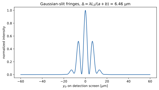
We now have a beam that reaches the slits, and the fraction that gets through. In Part 3 we will solve the problem for two slits numerically, dropping the assumption of Gaussian-shaped slits. There is no analytical solution to this next problem.
The full source for this series is on GitHub. The derivations, code, and prose are all mine. However, I did consult Claude to proofread and for help setting up the project and rendering equations.
A weekly email if there's something new.